Background
The purpose of these supplemental materials is to walk users through a few models and technical details associated with the {glmertree} package and provide references/supplemental reading for our poster. Refer to the Table of Contents (or scroll down) if you’re just here for references & recommended reading. Keep reading if you’re looking to learn how to run and extract parameters from these models. Please refer to the referenced works of Dr. Fokkema & colleagues for detailed interpretation of model output, etc.
For readability, code is included but can be shown/hidden by clicking show code.
load libraries
simulating data
For data privacy, I’m using simulated data to walk you through these models. If you don’t care about the simulation and just want to see model specification, keep reading; you’re in the right place! If you’re interested in knowing how I simulated the data, check out this blog post of mine.
I made a complex interaction term that would not be easily detected by a multilevel model (MLM), and showed how you would have to specify the fixed effects to appropriately approximate the data. This basically resulted in a 3-way interaction that would be highly unlikely to be theorized in multimodal approached, barring strong theoretical evidence or equally strong analyst capability (e.g., to draw associations from graphic exploration of the data).
We have 15 level 1 units for each level 2 unit and 71 level 2 units (labeled with id). The level 1 intercept of outcome is 4.25 with a main effect of 1.25 for x, 2.00 for z. The function also makes a nuisance variable w, which does not contribute to outcome at all.
show code
sim_dat <-
  simulate_nonlinear_intx(
    n = 15, ## number level 1 units at each level 2
    j = 71, ## number level 2 units
    intercept_lv1 = 4.25, ## intercept at level 1
    main_x = 1.25, ## main effect of x
    main_z = 2.00, ## main effect of z
    interaction1 = -4, ## interaction of x and z when product < 0
    interaction2 = 4, ## interaction of x and z when product >= 0
    residual_var_sd_lv1 = 2.00, ## standard deviation of residuals at level 1
    random_int_mean_lv2 = 0, ## mean of random intercept at level 2
    random_int_sd_lv2 = 1.00, ## standard deviation of random intercept at level 2,
    start_seed = 123 ## ensure you can reproduce
  )
GLMM trees should be able to find heterogeneity in the association of outcome and x (or z, it doesn’t matter) and explain differential effects of z and x without analyst knowledge of a complex higher-order interaction (i.e., n-way interactions when n > 2).
Fitting Generalized Linear Mixed Effects Model Regression (GLMM) Trees via {glmertree}
Specifying models with {glmertree} is similar to multilevel models (MLM) with {lme4}. However, rather than adding random effects with {lme4}, you specify the model as follows: forumla = outcome ~ fixed effects | random effects | splitting variables.
A second consideration when fitting GLMM trees is the model’s use of parameter instability tests; therefore, we need to account for cluster covariances in this process, so you want to specify the id variable to the cluster = id argument as well as in the specified formula. As far as I know, the current implementation only allows a 2 level structure, even if the MLM specified has more. The implications of inconsistent specification of data has not been examined to my knowledge.
Model 1: Fully Exploratory
Let’s run a very exploratory model here. This is everything but the kitchen sink: an intercept-only model, with random intercept for each level 2 unit, and allowing splits to be made by any of the variables in the data.
show code
tree_1 <-
  lmertree(
    data = sim_dat,
    formula =
      outcome ~ 1 | (1 | id) | x + z + w,
    cluster = id
  )
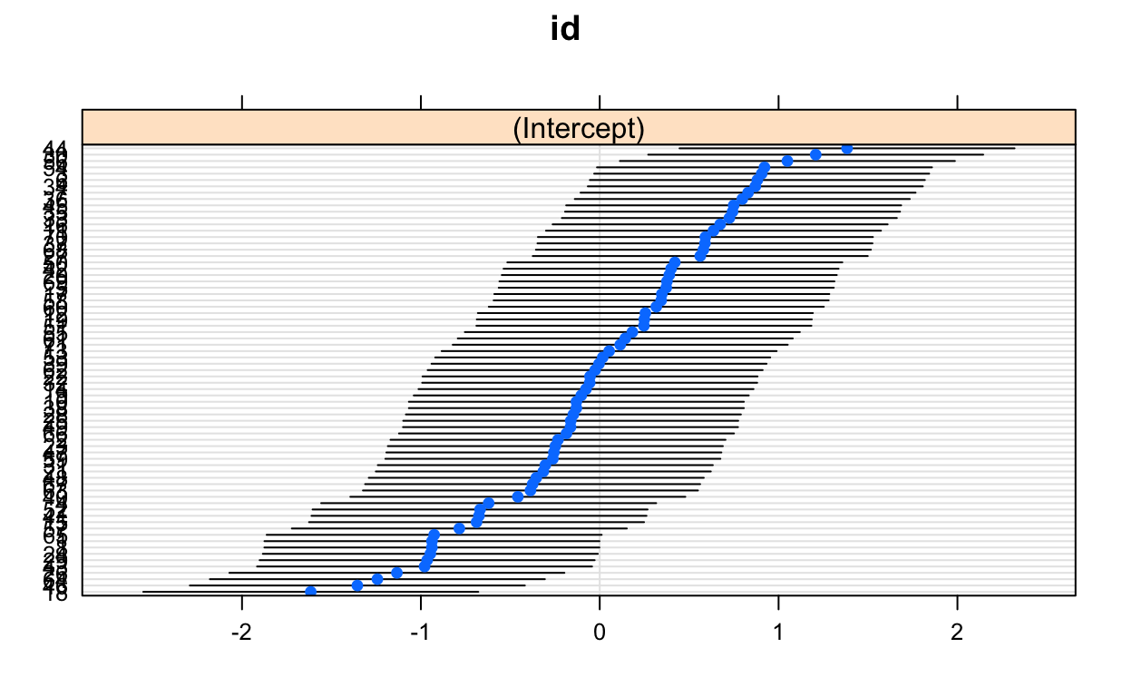
Let’s look at plotted results first. Here are the random effects, presented as a caterpillar plot. These random effects are showing the random intercept and surrounding variance for each id.
show code
custom_boxplot <-
  function(
    glmertree_object,
    write_labels = F
  ){
    format <- list(geom_edge(size = 1.2),
    geom_node_label(
      aes(label = splitvar),
      ids = "inner"),
    geom_node_plot(
        gglist = list(
          geom_boxplot(
            aes(y = outcome),
            size = 2),
          theme_minimal(base_size = 12),
          theme(
            axis.title.x = element_blank(),
            axis.text.x = element_blank(),
            axis.line.y = element_line(size = 1.5),
            panel.grid.minor.x = element_blank()
            )),
        shared_axis_labels = TRUE),
    geom_node_label(
      line_list =
        list(
          aes(label = splitvar),
          aes(label = paste('N = ' , nodesize)),
          aes(label = if_else(p.value < 0.001, "p < 0.001", paste0('p = ', round(p.value, 3))))),
      line_gpar = list(
        list(size = 15),
        list(size = 12),
        list(size = 12)),
      ids = "inner"),
    geom_node_label(
      aes(
        label = paste0("N = ", nodesize)
        ),
      ids = "terminal",
      line_gpar = list(list(size = 15))
      )
    )
    if (write_labels == T) {
      return(
        ggparty(glmertree_object$tree[1]) + geom_edge_label() + format
        )
    }
    else {return(ggparty(glmertree_object$tree[1]) + format)}
  }
Here’s a printed (instead of plotted) tree diagram. This diagram is too large to print easily, so it’s obviously more complex than we want (just scroll through this, I’m trying to emphasize the tree size!)
show code
tree_1$tree
Linear model tree

Model formula:
outcome ~ 1 | x + z + w

Fitted party:
[1] root
|   [2] z <= 1.05788
|   |   [3] x <= 0.92647
|   |   |   [4] z <= 0.37947
|   |   |   |   [5] x <= 0.66556
|   |   |   |   |   [6] x <= -1.81567: n = 10
|   |   |   |   |       (Intercept)
|   |   |   |   |          7.955253
|   |   |   |   |   [7] x > -1.81567
|   |   |   |   |   |   [8] z <= 0.1324
|   |   |   |   |   |   |   [9] x <= -0.89285
|   |   |   |   |   |   |   |   [10] z <= -0.50041
|   |   |   |   |   |   |   |   |   [11] z <= -1.26949: n = 12
|   |   |   |   |   |   |   |   |       (Intercept)
|   |   |   |   |   |   |   |   |           8.72907
|   |   |   |   |   |   |   |   |   [12] z > -1.26949: n = 33
|   |   |   |   |   |   |   |   |       (Intercept)
|   |   |   |   |   |   |   |   |          5.658304
|   |   |   |   |   |   |   |   [13] z > -0.50041: n = 35
|   |   |   |   |   |   |   |       (Intercept)
|   |   |   |   |   |   |   |            3.1839
|   |   |   |   |   |   |   [14] x > -0.89285
|   |   |   |   |   |   |   |   [15] x <= 0.23029
|   |   |   |   |   |   |   |   |   [16] z <= -0.89841
|   |   |   |   |   |   |   |   |   |   [17] x <= -0.26504: n = 42
|   |   |   |   |   |   |   |   |   |       (Intercept)
|   |   |   |   |   |   |   |   |   |          4.032858
|   |   |   |   |   |   |   |   |   |   [18] x > -0.26504: n = 47
|   |   |   |   |   |   |   |   |   |       (Intercept)
|   |   |   |   |   |   |   |   |   |          1.914251
|   |   |   |   |   |   |   |   |   [19] z > -0.89841: n = 155
|   |   |   |   |   |   |   |   |       (Intercept)
|   |   |   |   |   |   |   |   |          4.057118
|   |   |   |   |   |   |   |   [20] x > 0.23029: n = 99
|   |   |   |   |   |   |   |       (Intercept)
|   |   |   |   |   |   |   |          4.654456
|   |   |   |   |   |   [21] z > 0.1324: n = 77
|   |   |   |   |   |       (Intercept)
|   |   |   |   |   |          5.229926
|   |   |   |   [22] x > 0.66556: n = 72
|   |   |   |       (Intercept)
|   |   |   |          6.074059
|   |   |   [23] z > 0.37947: n = 164
|   |   |       (Intercept)
|   |   |          6.806958
|   |   [24] x > 0.92647
|   |   |   [25] z <= 0.56022
|   |   |   |   [26] z <= -0.76973
|   |   |   |   |   [27] x <= 1.33385: n = 19
|   |   |   |   |       (Intercept)
|   |   |   |   |           8.61226
|   |   |   |   |   [28] x > 1.33385: n = 23
|   |   |   |   |       (Intercept)
|   |   |   |   |          12.99779
|   |   |   |   [29] z > -0.76973
|   |   |   |   |   [30] z <= 0.31077
|   |   |   |   |   |   [31] z <= -0.31704: n = 33
|   |   |   |   |   |       (Intercept)
|   |   |   |   |   |          8.141308
|   |   |   |   |   |   [32] z > -0.31704: n = 39
|   |   |   |   |   |       (Intercept)
|   |   |   |   |   |          6.283608
|   |   |   |   |   [33] z > 0.31077: n = 21
|   |   |   |   |       (Intercept)
|   |   |   |   |          9.217174
|   |   |   [34] z > 0.56022: n = 26
|   |   |       (Intercept)
|   |   |          12.82893
|   [35] z > 1.05788
|   |   [36] x <= 1.13431
|   |   |   [37] z <= 1.95389
|   |   |   |   [38] x <= -0.99028: n = 16
|   |   |   |       (Intercept)
|   |   |   |          14.03631
|   |   |   |   [39] x > -0.99028
|   |   |   |   |   [40] x <= 0.53007: n = 70
|   |   |   |   |       (Intercept)
|   |   |   |   |          9.506037
|   |   |   |   |   [41] x > 0.53007: n = 30
|   |   |   |   |       (Intercept)
|   |   |   |   |          12.58756
|   |   |   [42] z > 1.95389: n = 17
|   |   |       (Intercept)
|   |   |          15.56201
|   |   [43] x > 1.13431
|   |   |   [44] z <= 1.58438: n = 15
|   |   |       (Intercept)
|   |   |          16.82666
|   |   |   [45] z > 1.58438: n = 10
|   |   |       (Intercept)
|   |   |          23.86421

Number of inner nodes:    22
Number of terminal nodes: 23
Number of parameters per node: 1
Objective function (residual sum of squares): 5187.452
It looks like our model has identified too many splits for this to extract meaningful interpretations We gain knowledge that x and z are the variables that contribute to the outcome. The model is never presenting w as a variable influencing splitting when there is so much more heterogeneity in levels of z and x. We can prevent the model from building such a large tree with the maxdepth parameter. We’ll get broader strokes of the process, but will be less likely to overfit the data.
NOTE: For visual consistency when knitting the document, I actually wrote a custom function (above) to make {ggparty} plotting easy across the project, but you can also just use plot(tree_1, which = 'tree').
There are two ways we could begin working to make results which can be interpreted. One is to just tune hyperparameters. The other is to add fixed effects, which we’ll do later.
Model 2: Modify hyperparameters
Hyperparameters are parameters that can be specified by the researcher; these parameters influence the estimation of the parameters in the model. These are common for machine learning, and those relevant to GLMM trees are any that are relevant to decision trees or parameter instability tests (see {partykit}).
I’ll point you towards a few and their defaults.
bonferroni = TRUE: Bonferroni corrects p-values. Recommended to leave on.alpha = 0.05: p-value indicated significant parameter stability (e.g.,alpha = 0.001).minsize = NULL: the minimum cases allowed in the terminal node. The larger you make this, the more of the sample has to be in a node for you to trust there is generalize-able heterogeneity and not just noise in your data (e.g.,minsize = 0.10*nrow(your_data_set))trim = NULL: this specifies the percentage (if < 0) or number (if > 0) of outliers to be be omitted from the parameter instability tests. This is done to prevent undue influence of outliers, and does not influence group assignment/splitting; it is just used in testing.maxdepth = Inf: the depth of the tree that’s allowed to grow. This functionally decreases the level of interactions you allow the data to find.
These should be tuned carefully and resulting models are ideally discussed with content experts and compared to prior research for validity.
Let’s re-run this with some more stringent hyperparameters and see how the model explains relation of x, z, and outcome. Since this grew such a deep tree, that’s the first hyperparameter I’ll tune.
show code
tree_2 <-
  lmertree(
    data = sim_dat,
    formula =
      outcome ~ 1 | (1 | id) | w + z + x,
    cluster = id,
    maxdepth = 3,
  )
show code
custom_boxplot(tree_2, write_labels = T)

Model 3: add fixed effects
The p < 0.001 on the nodes indicate the parameter instability test is significant and the 2 models explain more variance in the data than 1 model (repeated at subsequent nodes, too). The value for the test can be found via partykit::sctest.modelparty(glmertree_model$tree, type = c("chow"), asymptotic = F) when your model name is glmertree_model. If these were barely p < 0.05, I would likely tune this next. Also, this model looks fairly interprettable.
This is saying z being ~1 standard deviation above its mean, the outcome is highest. When it’s lower than that, it’s lower. Within these cases, outcome appears to be higher when x is higher. This suggests an interaction of x and z. We could now see what the relationship of x to the outcome is for different values of z, by adding it as a fixed effect.
show code
tree_3 <-
  lmertree(
    data = sim_dat,
    formula =
      outcome ~ x | (1 | id) | w + z + x,
    cluster = id,
    maxdepth = 3,
    trim = 0.1
  )
show code
custom_scatter_lm <-
  function(
    glmertree_object
  ){
    ggparty(glmertree_object$tree[1]) +
    geom_edge(size = 1.2) +
    geom_edge_label() +
    geom_node_label(
      aes(label = splitvar),
      ids = "inner") +
  geom_node_plot(
      gglist = list(
        geom_point(
          aes(y = outcome, x = x),
          size = 2),
        geom_smooth(method = 'lm', aes(y = outcome, x = x)),
        theme_minimal(base_size = 30),
        theme(
          axis.line.y = element_line(size = 1.5),
          panel.grid.minor.y = element_blank(),
          axis.text.x = element_text(size = 12)
          )),
      shared_axis_labels = TRUE,
      scales = 'free_x')+
  geom_node_label(
    line_list =
      list(
        aes(label = splitvar),
        aes(label = paste('N = ' , nodesize)),
        aes(label = if_else(p.value < 0.001, "p < 0.001", paste0('p = ', round(p.value, 3))))),
    line_gpar = list(
      list(size = 20),
      list(size = 20),
      list(size = 20)),
    ids = "inner") +
  geom_node_label(
    aes(
      label = paste0("N = ", nodesize)
      ),
    ids = "terminal",
    line_gpar = list(list(size = 20))
  ) +
      labs(caption = 'note x axes are free') +
      theme(plot.caption = element_text(size = 20))
  }
show code
custom_scatter_lm(tree_3)

We now see a more nuanced description of the relationship of x to outcome at different levels of z, and the subgroups are slightly different than in tree_2. When z is large, we see larger average outcome (i.e., intercept) than when z is lower. On both halves of the plot, it looks like the relationship of x and outcome is negative when x < 0, but is positive when x > 0. Let’s put these onto one plot and see what it looks like.
Visualizing the Data
show code
figure_1a <-
  sim_dat %>%
  mutate(node = factor(as.vector(predict(tree_3, type = 'node')))) %>%
  ggplot(aes(x = x, y = outcome, group = node, color = node)) +
  geom_point(alpha = 0.6) +
  geom_smooth(method = 'lm') +
  theme_minimal() +
  project_theme +
  labs(
    title = 'Model fit by glmertree',
    ) +
  theme(plot.subtitle = element_text(size = 15))
figure_1a

The plot above shows that we created 4 linear models appear to explain the data well. Let’s see actual parameter estimates.
Viewing Model Parameters
Discontinuous Linear Models
The parameters from these models can be represented as discontinuous linear models with random effects offsets by calling summary(tree_3$tree).
show code
summary(tree_3$tree)
$`3`

Call:
lm(formula = outcome ~ x, offset = .ranef)

Residuals:
    Min      1Q  Median      3Q     Max
-8.0329 -1.8072 -0.0501  1.7780 10.0277

Coefficients:
            Estimate Std. Error t value Pr(>|t|)
(Intercept)   3.7350     0.2059  18.138  < 2e-16 ***
x            -1.4000     0.2322  -6.029 3.62e-09 ***
---
Signif. codes:  0 '***' 0.001 '**' 0.01 '*' 0.05 '.' 0.1 ' ' 1

Residual standard error: 2.602 on 418 degrees of freedom
Multiple R-squared:  0.1456,    Adjusted R-squared:  0.1435
F-statistic: 71.21 on 1 and 418 DF,  p-value: 5.298e-16


$`4`

Call:
lm(formula = outcome ~ x, offset = .ranef)

Residuals:
    Min      1Q  Median      3Q     Max
-7.9603 -1.6546  0.0238  1.5724  7.9335

Coefficients:
            Estimate Std. Error t value Pr(>|t|)
(Intercept)   3.9118     0.1995   19.61   <2e-16 ***
x             3.4500     0.2035   16.95   <2e-16 ***
---
Signif. codes:  0 '***' 0.001 '**' 0.01 '*' 0.05 '.' 0.1 ' ' 1

Residual standard error: 2.499 on 454 degrees of freedom
Multiple R-squared:  0.4142,    Adjusted R-squared:  0.4129
F-statistic:   321 on 1 and 454 DF,  p-value: < 2.2e-16


$`6`

Call:
lm(formula = outcome ~ x, offset = .ranef)

Residuals:
    Min      1Q  Median      3Q     Max
-6.9413 -2.1484 -0.0186  1.6858  7.4166

Coefficients:
            Estimate Std. Error t value Pr(>|t|)
(Intercept)   8.0073     0.4199  19.070   <2e-16 ***
x            -3.4074     0.4446  -7.664    2e-11 ***
---
Signif. codes:  0 '***' 0.001 '**' 0.01 '*' 0.05 '.' 0.1 ' ' 1

Residual standard error: 2.744 on 90 degrees of freedom
Multiple R-squared:  0.4176,    Adjusted R-squared:  0.4111
F-statistic: 64.54 on 1 and 90 DF,  p-value: 3.48e-12


$`7`

Call:
lm(formula = outcome ~ x, offset = .ranef)

Residuals:
    Min      1Q  Median      3Q     Max
-6.3134 -2.3014 -0.5595  2.5627 10.5835

Coefficients:
            Estimate Std. Error t value Pr(>|t|)
(Intercept)   7.5139     0.7371  10.194  < 2e-16 ***
x             6.8414     0.6895   9.923 2.42e-16 ***
---
Signif. codes:  0 '***' 0.001 '**' 0.01 '*' 0.05 '.' 0.1 ' ' 1

Residual standard error: 3.529 on 95 degrees of freedom
Multiple R-squared:  0.5026,    Adjusted R-squared:  0.4973
F-statistic: 95.98 on 1 and 95 DF,  p-value: 4.491e-16
Multilevel Models
Alternatively, they could be presented as multilevel models summary(tree_3$lmer).
show code
summary(tree_3$lmer)
Linear mixed model fit by REML ['lmerMod']
Formula: outcome ~ .tree + .tree:x + (1 | id)
   Data: data
Weights: .weights
Control: lmer.control

REML criterion at convergence: 5224.1

Scaled residuals:
    Min      1Q  Median      3Q     Max
-2.9480 -0.6594 -0.0312  0.6311  3.8841

Random effects:
 Groups   Name        Variance Std.Dev.
 id       (Intercept) 0.8057   0.8976
 Residual             7.4246   2.7248
Number of obs: 1065, groups:  id, 71

Fixed effects:
            Estimate Std. Error t value
(Intercept)   3.7350     0.2439  15.314
.tree4        0.1768     0.3128   0.565
.tree6        4.2723     0.4804   8.894
.tree7        3.7789     0.6180   6.115
.tree3:x     -1.4000     0.2476  -5.653
.tree4:x      3.4500     0.2267  15.216
.tree6:x     -3.4074     0.4514  -7.549
.tree7:x      6.8414     0.5418  12.627

Correlation of Fixed Effects:
         (Intr) .tree4 .tree6 .tree7 .tr3:x .tr4:x .tr6:x
.tree4   -0.637
.tree6   -0.415  0.328
.tree7   -0.319  0.250  0.166
.tree3:x  0.710 -0.558 -0.366 -0.280
.tree4:x  0.004 -0.576 -0.010 -0.002  0.006
.tree6:x -0.004  0.004  0.651  0.006 -0.004 -0.003
.tree7:x -0.005  0.005 -0.001 -0.814 -0.001  0.000 -0.003
Going Beyond Significance
We also see, though, that the 2 models formed approximately when x < 0 overlap with one another, as do the 2 models when x > 0 (approximately). This is where we would call in researchers that know the field. We would discuss the evidence in the data, compared to the theoretical possibilities of 4 versus 2 groups.
These 4 groups may be phenomena observed or the way the model is formed may influence the fact that we have 2 parallel lines. This is also clear from the intercepts and slopes presented in summary(tree_3$tree). You see, since the tree structure is dependent upon the first split, the parameter instability tests do not go across branches to see if groups could be recombined to increase model fit
If an analyst were working with a theorist, they should discuss the implications of these 4 groups and find some way to demonstrate validity of 4 over 2 (as Occum’s Razor would suggest 2 is more likely than 4). If an analyst were working alone, I would suggests following up this with one final parameter instability test, comparing models with individual negative slopes to a single negative slope. Then, repeating this for 1 vs. 2 positive slopes.
Visually, two groups would look like this
show code
sim_dat %>%
  mutate(node = factor(as.vector(predict(tree_3, type = 'node'))),
         dichot_node = factor(if_else(node %in% c(4,7), 1, 0))
         ) %>%
  ggplot(aes(x = x, y = outcome, group = dichot_node, color = dichot_node)) +
  geom_point() +
  geom_smooth(method = 'lm') +
  theme_minimal() +
  project_theme +
  labs(
    title = 'Collapsing Nodes',
    ) +
  theme(plot.subtitle = element_text(size = 15))

This looks like a reasonable model, which could explain not only the sample, but the population as it does for us (based on its similarity to the method of simulation). Random forest modifications could be useful to preventing such overfitting, but that will have to wait for another article.
References & Recommended Reading
Bates, D., Maechler, M., Bolker, B., & Walker, S. (2015). Fitting Linear Mixed-Effects Models Using lme4. Journal of Statistical Software, 67(1), 1-48. doi:10.18637/jss.v067.i01.
Fokkema, M., Edbrooke-Childs, J., & Wolpert, M. (2020). Generalized linear mixed-model (GLMM) trees: A flexible decision-tree method for multilevel and longitudinal data. Psychotherapy Research, 31(3), 329-341.
Fokkema, M., Smits, N., Zeileis, A., Hothorn, T., & Kelderman, H. (2018). Detecting treatment-subgroup interactions in clustered data with generalized linear mixed-effects model trees. Behavior research methods, 50(5), 2016-2034.
Hothorn, T. & Zeileis, A. (2015). partykit: A Modular Toolkit for Recursive Partytioning in R. Journal of Machine Learning Research, 16, 3905-3909.
Hothorn, T., Hornik, K., & Zeileis, A. (2006). Unbiased recursive partitioning: A conditional inference framework. Journal of Computational and Graphical statistics, 15(3), 651-674.
Hulleman, C. S., Godes, O., Hendricks, B. L., & Harackiewicz, J. M. (2010). Enhancing interest and performance with a utility value intervention. Journal of educational psychology, 102(4), 880.
Borkovec, M. & Madin, N. (2019). ggparty: ‘ggplot’ Visualizations for the ‘partykit’ Package. R package version 1.0.0.
Villanueva, I., Husman, J., Christensen, D., Youmans, K., Khan, M.T., Vicioso, P., Lampkins, S. and Graham, M.C., 2019. A Cross-Disciplinary and Multi-Modal Experimental Design for Studying Near-Real-Time Authentic Examination Experiences. JoVE (Journal of Visualized Experiments), (151), p.e60037.
Wickham et al., (2019). Welcome to the tidyverse. Journal of Open Source Software, 4(43), 1686,
Zeileis, A. (2001). strucchange: Testing for structural change in linear regression relationships. R News, 1(3), 8-11.
Zeileis, A., Hothorn, T., & Hornik, K. (2008). Model-based recursive partitioning. Journal of Computational and Graphical Statistics, 17(2), 492-514.